X 服务器格式，翻译和成员属性

译者：hxhgxy  来源：http://blogs.msdn.com/excel
发表于：2006年7月7日

PivotTables X: Server formatting, translations, member properties
数据透视表 X：服务器格式，翻译，成员属性

In this post I’ll walk you through three Analysis Services features that we now support in Excel PivotTables – server formatting, translations, and member properties. One thing to keep in mind as you read is that since all these are defined in Analysis Services (i.e. on a server), every PivotTable created that pulls data from Analysis Services will get the benefit of these features without the PivotTable author or user needing to do anything.
在本文里，我将带领你浏览我们现在在Excel 数据透视表里支持的Analysis Services功能——服务器格式，翻译和成员属性。你在阅读的时候请牢记一件事，因此这些都是在Analysis Services（例如在服务器上）上定义的，从Analysis Services获得的数据而创建的每个数据透视表将会从中获益而不需要数据透视表作者或者用户去做任何事情。

Server formatting
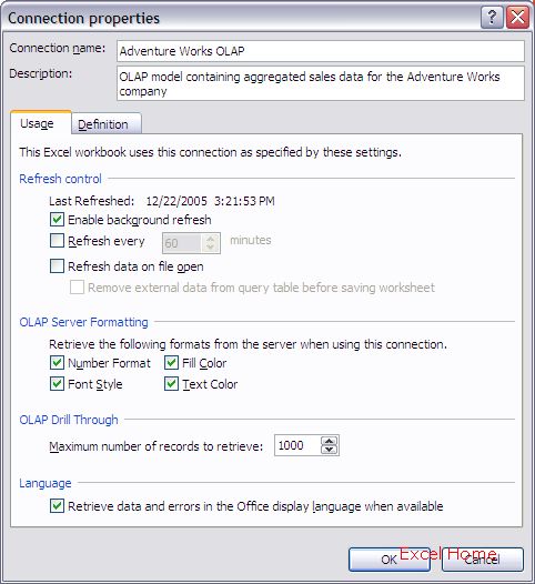
When designing a model in Analysis Services, formatting can be associated with values. Excel PivotTables will display this formatting by default (you can control it in the connection properties dialog for the connection being used by the PivotTable, so if you want to turn off the formatting, you can).
服务器格式
在Analysis Services设计模型时，设计数据的同时也可以设置格式。Excel数据透视表将会默认地显示这些格式（你可以在连接属性对话框里控制它，因此如果你想要关闭格式的话，你可以做到）

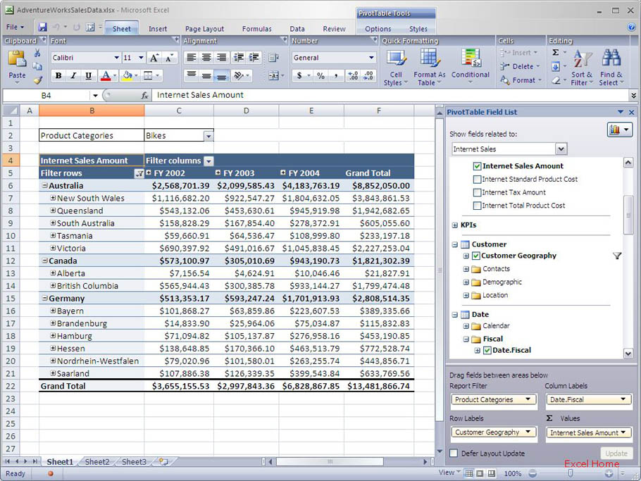
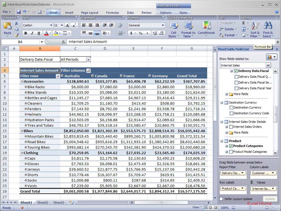
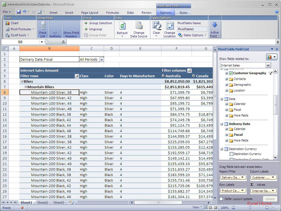
Here is an example of a PivotTable displaying number formatting as defined on the server – in this case dollars with two decimals. As you add fields to the Values area of the PivotTable, the formatting is done automatically.
这里有个例子，数据透视表显示服务器上设计的数字格式——在本例中，为带两位小数位数的美元。当你添加字段到数据透视表的数值区域时，格式会自动完成。

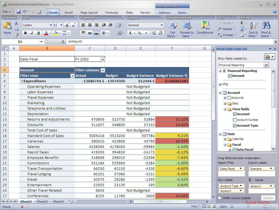
The next screenshot illustrates fill color formatting defined on the server. In this case, the formatting is actually based on a rule (MDX expression), setting different fill colors based on the value in each cell. You can think of this as conditional formatting defined in Analysis Services. Again, the user didn’t have to do anything but add the fields to the PivotTable to get server defined conditional formatting based on centralized business rules. In the example, the rule colors cells with acceptable values green, cells with unacceptable values red and cells with values in between are colored yellow.
下一张截图示范在服务器上设计的填充色格式。在这种情形中，格式实际上是基于一个规则（MDX表达式）的，基于每个单元格的数值设置不同的填充颜色。你可以将其看作是定义在Analysis Services里的条件格式。同样，用户不必做任何事情，只是添加该字段到数据透视表，以获取服务器基于集中的业务规则定义的条件格式而已。在该例子里，颜色规则是，可接受的数值为绿色，不可接受的数值的单元格为红色，位于两者之间的数值单元格填充为黄色。

This is pretty powerful … business logic can be defined in an Analysis Services model, and everyone that views the data sees that business logic in their spreadsheet without having to do anything except add fields to their PivotTable.
这功能真是非常强大……业务逻辑可以在Analysis Services模型里定义，然后查看数据的每个人在他们的电子表格里都可以看到该业务逻辑，而不必做任何事情，除了添加字段到他们的数据透视表。

Translations
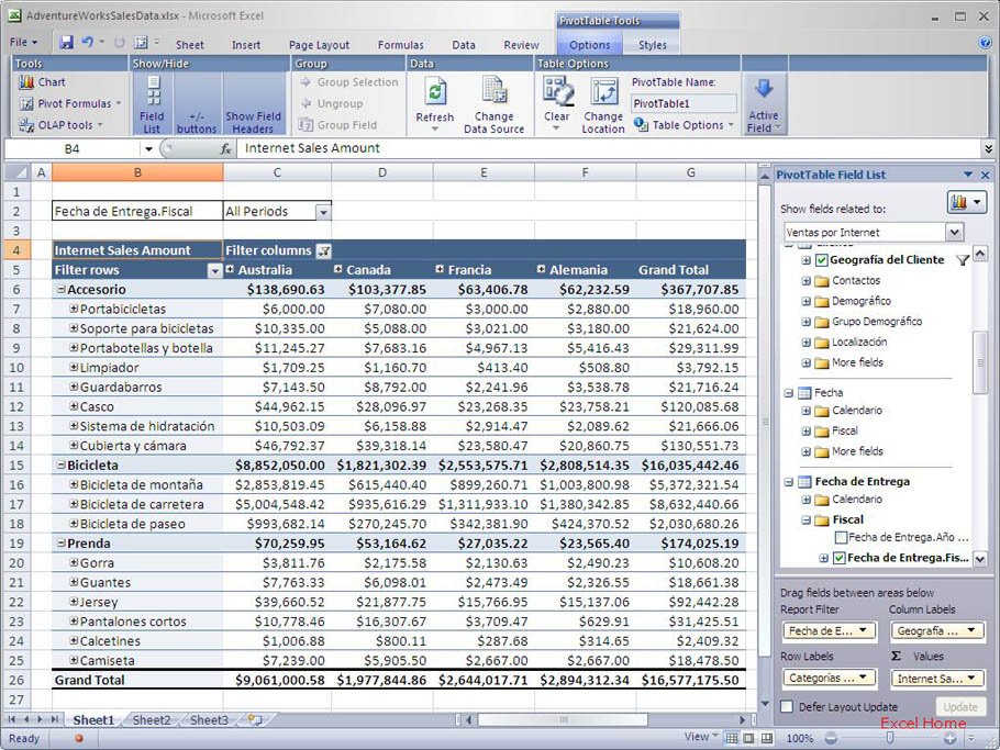
For global companies, it is important that employees and customers in different countries can access corporate data in their native language. Analysis Services 2005 offers a new “translations” feature that enables you to have multiple translations of the same model. For example, you might have you product catalog available in English, French, German and Spanish. Excel 12 PivotTables expose these translations in the report itself as well as in the field list. Based on the language settings on the machine where Excel is running, Excel will automatically pick the same language if it exists on the server. If that language does not exist, the default language specified on the server will be picked. You can override this automatic behavior by specifying a locale identifier in the connection information for the PivotTable and thereby force the use of a specific language.
翻译
对于一个全球性公司，不同国家的员工和客户能够用其母语访问公司数据是非常重要的。Analysis Services 2005提供了一个新功能“翻译”，让你可以使同一个模型有多种翻译。例如，你的产品目录可能有英语的，法语的，德语的和西班牙语的。Excel 12数据透视表不但将这些翻译出现在报表本身，而且也出现在字段列表里。基于Excel运行的机器上的语言设置，如果该语言在服务器上也存在的话，Excel将自动选择相同的语言。如果该语言不存在，那么服务器上指定的缺省语言就会被选上。你可以忽视该自动行为，为数据透视表在连接信息里指定一个当地标识符，强行要求使用指定的语言。

Let’s look at an example. Here is a PivotTable displaying the English translations of the server model, which is what you would see if you open the Excel file on a machine running English Excel 12.
我们来看一个示例。这里是一个显示从服务器模型来的英语版数据透视表，如果你在一个英语版的Excel 12运行的机器上打开Excel文件的话，这也是你想看到的。

Now, I’ll pick a different connection file pointing to the same server model. This connection file specifies that I want the Spanish translations.
现在，我将选择一个不同的文件连接到同一个服务器模型。该连接文件指定我需要西班牙版本。

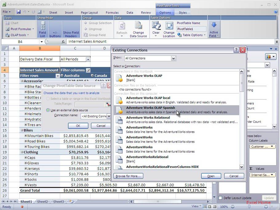
In this case I chose a new connection, but the same thing would have happened had I opened the Excel file on a Spanish machine running Excel 12.
在本例中，我关闭了一个新连接，但是如果我在一个西班牙语机器运行的Excel 12中打开该Excel文件时，同样的事情也会发生。

Member properties
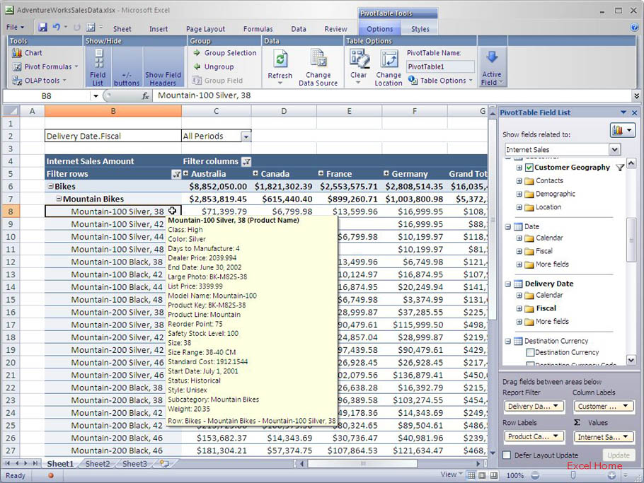
When analyzing data, it can be very helpful to get at additional information about an item to make better decisions. For example, if you’re looking at product sales, it might be very helpful to be able to quickly look up all the information on a specific product to better understand the sales amount for that product. Member properties in Analysis Services allow you to do just that. Excel 12 PivotTables expose member properties in tooltips, so all you have to do is to hover over the product that you want more information on, and this information will be displayed in a tooltip.
成员属性
在分析数据时，如果能获取某个项目的额外信息的话，那么对于做一个更好的决定是很有帮助的。例如，如果你正在查看产品销售情况，如果能够快速查看某个具体产品的所有信息，以更好地理解该产品的销售量，那么会很有帮助的。Analysis Services里的成员属性允许你实现这个。Excel 12数据透视表将成员属性显示在工具提示里面，因此你所有要做的事情只是将鼠标移到你需要更多信息的产品之上，该信息就会被显示在工具提示上。

The member properties can also be added inside the PivotTable itself when you need to print the information or just have it be visible all the time. Here is what that looks like.
成员属性也可以添加到数据透视表本身内部，当你需要打印该信息或者只是想让它时时可见。这是它的样子。

Finally, the Excel Object Model can be used to make member properties display instead of the members those properties pertain too. For example, if you have quarters represented as “First Quarter 2004”, “Second Quarter 2004”, etc., you can define a member property with abbreviated names like “Q1 04”, “Q2 04” etc. and set a flag to show the properties when the field is placed in the column area, making the report more readable (less wide).
最后，Excel对象模型可以用来显示成员属性，而不是拥有那些属性的成员。例如，如果你有一些季度，表现为“First Quarter 2004”，“Second Quarter 2004”，等等，那么你可以定义成员属性为一些缩写的名称如“Q1 04”，“Q2 04”等，并且当放置该字段到列区域时设置一个标志以显示该属性，这样可以使报表更易读（列宽窄一些）。

Published Thursday, January 05, 2006 5:40 PM by David Gainer

注：本文翻译自http://blogs.msdn.com/excel，原文作者为David Gainer(a Microsoft employee)，Excel home授权转载。严禁任何人以任何形式转载，违者必究。