数据透视图
译者:snood 来源:http://blogs.msdn.com/excel
发表于:2006年7月7日
Charting V – PivotCharts
数据透视图
Whenever we talk to users about PivotCharts, the first request we hear is that they behave more like regular charts. In previous versions, PivotCharts had very limited layout and formatting options. In addition, if you refreshed the PivotTable that the PivotChart was based upon, the PivotChart would lose whatever formatting it had. We heard from many users that they would often just create regular charts instead of PivotCharts, since could be problematic As PivotTables and charts changed in Excel 2007, we made sure PivotCharts changed along with them – with a key goal being that they became more consistent.
只要我们和用户谈论有关数据透视图,我们听到的第一个要求是,能像正常图表一样使用. 以前的版本, 数据透视图只有非常有限的布局和格式选项。此外,如果更新数据透视图的基础:数据透视表,它就会丢失所有已设置的格式. 我们听到许多用户往往只能用正常图表代替数据透视图。因为这些问题,在Excel 2007中的数据透视表和数据透视图有所改变,我们相信数据透视图改变的主要目标是让图表变得更加一致。
Formatting
PivotCharts in Excel 2007 can have all the same formatting as regular charts, including all the layouts and styles talked about in previous posts. You can move and resize chart elements, or change formatting of individual data points. One of the few restrictions that we did not have time to address in this version is the one on chart types – you still can’t create scatter, bubble, or stock PivotCharts.
If you refresh the data for your PivotChart, the chart updates and the formatting does not change. Any new series or data points will be formatted to match the style or series as appropriate. As a result, you can easily make PivotCharts for presentation or publication.
Furthermore, PivotChart will remember formatting across pivots. If you set the colour of the series or a particular data point to red, then change the pivot so your data is no longer showing, the red band is gone as well. If you bring the data back into view, the red colour returns.
格式
Excel2007数据透视图和正常图表一样有许多相同格式,包括前面讨论的所有的设计风格和图表类型。你可以移动和改变图表元素,或变更单个数据系列的格式. 少数的限制中的一项是,我们没有时间处理图表类型:在这个版本中还是不能创建散点图、气泡图、股票图等数据透视图.
如果你更新数据透视图、数据会更新而图表格式不会改变. 任何新的数据系列或数据点格式将设置成相同的风格. 因此,很容易创建数据透视图来制作幻灯片或出版物。
此外, 数据透视图将通过字段记忆格式. 如果你设定某系列或某数据点的颜色为红色,那么当你改变透视关系不再显示此数据系列,红色系列消失了;如果你再设置显示该字段时,红色系列又回来了。
PivotTable Field List
PivotCharts use the same field list as PivotTables. Just as with PivotTables, you can click the checkboxes for the fields you are interested in, and they will be reasonably laid out as a PivotChart. You can also drag the fields around from region to region to pivot the PivotChart. The field list also provides access to field settings such as how to summarize the data.
数据透视图字段列表
数据透视图使用和数据透视表相同的字段列表. 如同数据透视表,你可以点击字段列表来插入,并创建合适的数据透视图. 你还可以拖放字段,从数据透视图的一个区域移动另一个区域. 字段列表还规定了字段取数,例如如何汇总数据.
PivotChart Filter Pane
The PivotChart filter pane is a new task pane that enables you to filter PivotCharts. In previous versions, filters were accessed from buttons in the PivotChart, but removed these so they didn’t affect the layout of the PivotChart. The filter pane has the same filter capabilities as for PivotTables. See filtering in PivotTables for details. Below is a shot of the PivotChart field list and Filter task pane.
数据透视图筛选窗格
数据透视图筛选窗格是一个新的任务窗口,便于进行数据透视图筛选。以前的版本,是使用数据透视图的筛选按钮,去掉这些按钮并不影响数据透视图的布局。筛选窗口和数据透视表具有相同的筛选功能。详细的数据透视表筛选参见(http://blogs.msdn.com/excel/archive/2005/12/20/506172.aspx). 下面是一张关于数据透视图的字段和筛选窗口的截图。
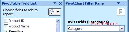
(Click to enlarge)
Published Wednesday, April 19, 2006 11:57 PM by David Gainer
注:本文翻译自http://blogs.msdn.com/excel ,原文作者为David Gainer(a Microsoft employee),Excel Home 授权转载。严禁任何人以任何形式转载,违者必究。