Tables Part 4_自动筛选的改进（二）_Excel 2007新知

译者：lfspecter  来源：http://blogs.msdn.com/excel
发表于：2006年7月7日

In the spirit of completeness, Excel 12 also provides text-based filters for working with non-numeric columns.

为了力求功能的完整，excel 12 对没有数字的列也提供了文本筛选功能

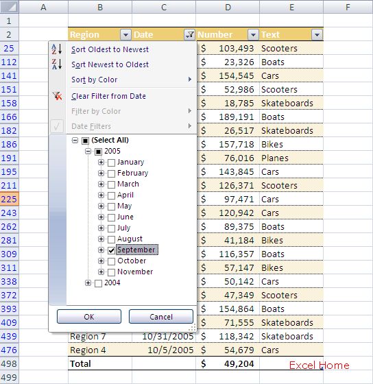
Another feature for date-based columns is that the filter dropdown groups dates by day/month/year rather than displaying a flat list of dates so that it’s easier to drill-down and pick a specific series of dates. If you wanted to select all of the dates in a particular month for instance, you can do so in two clicks.
对日期筛选的另一个特点是在筛选的下拉列中日期是按年月日排列而不是简单的日期的排列，这样，如果要筛选一个特定的日期系列就容易多了。比如，当你想筛选日期列中的某个特定的月时，点击鼠标两次就可以完成了。

In Excel 12, we have gone beyond the ability to filter on values in cells. We now also support the ability to filter by colour color. For example, if I have a table of data I’m working with and I’m using orange and red fill as a way to mark rows that need special attention, I may want to just filter to see everything I have marked red. To set that up is just a few clicks.
在excel12中，我们能做的已超出了对单元格中数值的筛选，现在我们还能通过给单元格涂颜色进行筛选。例如，当我处理一张工作表的数据时，我用桔黄色和红色来填充某些需要特殊关注的行，这样我可以通过筛选来查看所有我标记了红色的内容，几次点击就可完成。

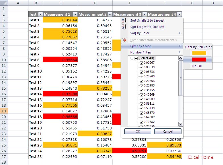
Filter by colour allows you to filter by font colour as well as cell fill colour. In addition, it also recognizes conditional formats on cells including regular formatting, gradient fills, and conditional formatting icon sets (which I discussed in previous posts here and here).
颜色筛选不仅支持单元格颜色，也支持字体颜色。另外，也能识别单元格的条件格式，包括正常格式，斜体填充和条件格式图标设置。（以前的贴中已提到过）

In the same way that we have enabled filtering by colour, we have enabled sorting by colour which, predictably enough, allows you to sort your data based on cell or background colour. I will run through an example of that in the next post.
与颜色筛选一样，我们同样可以用颜色进行排序，足够的颜色可以使你基于单元格或背景颜色排序。下一贴中我将举例演示。

Excel 12 makes it a bit easier to notice when a table has been filtered or sorted as well as easier to figure out what the sort or filter is. For any column that has a filter set, Excel changes the filter dropdown icon to denote its filter state. The same thing happens, although a different icon is used, for columns that have been sorted. In the screenshot below, you can spot which columns were used to sort and filter the table. In addition, you can get more information by hovering the mouse over the icon … Excel will show a tooltop that describes the sort and filter state of the column.
当一个列表处于筛选或排序状态时，Excel 12 使用户更容易注意到并看出是哪一种筛选或排序。因为每一列都有一个筛选标识，excel 通过改变筛选下拉图标来指示筛选状态。同样的，通过在被筛选的数据列使用的不同的图标，下图中，你可以指出哪一列被用来筛选或排列整个列表。另处你可以移动鼠标指向图标从而得到更多信息……Excel 将在你鼠标所指处显示筛选排列状态。

Filter buttons and tooltip
As in previous versions, a sort or filter is only applied at the time the sort or filter is created (or a query is refreshed if the table is connected to external data). This is necessary so that data doesn’t shift around or “disappear” as you are editing it. Of course there will be times when a sort or filter becomes stale and needs to be reapplied, like after you have copied and pasted a bunch of new records to the bottom of a table or range. Excel 12 makes it easy to reapply all sort and filter conditions on a table via a single click of a ribbon button.
和以前的版本相同，排列或筛选的命令只在排列或筛选被建立时有效（当列表有外部数据链接时需要刷新）。这样才不会在你编辑数据时造成数据移动或消失。当然，这样就会偶尔出现一种情形：一个排序或筛选过时而需重新执行，比如，当你复制粘贴了大量的数据到一个列表或一个区域的底部时。Excel 12使能够通过点击一次工具按钮来重新执行筛选或排列。

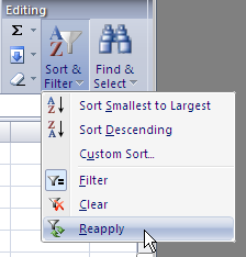
Reapply Command on the Ribbon
As you can see from the screenshot above, it also takes a single click to remove all filters from all columns in a table.
如上图所示，取消筛选和排列也只需击鼠标一次即可完成

The last thing I want to mention before closing is that everything I have discussed here can be used without the table feature, however there are certain advantages to using them in conjunction with tables. Each table has its own AutoFilter whereas the sheet can only have a single AutoFilter, so if you need to filter more than one dataset on a sheet, than tables are your only option. Similarly, tables also remember their own sort conditions, so if you need the ability to maintain multiple sort states across a sheet than tables will do the trick.
在结束前我想提到的最后一件事是我所说的所有功能可以在不涉及列表特性的前提下使用，当然和列表结合后还会有一定的优势。虽然工作表只能有一个自动筛选，但是每个列表都可以有自己的自动筛选。 所以当你在工作表中需要不止一个数据集时，列表是你唯一的选择。与此类似，列表也记忆自己的排序条件，所以如果你需要在整个工作表中进行多重排列时， 可以借助列表来实现。

Next time, more on sorting.
下次，我们将继续讲解排序

Published Tuesday, November 01, 2005 3:30 PM by David Gainer

注：本文翻译自http://blogs.msdn.com/excel ，原文作者为David Gainer（a Microsoft employee)，Excel Home 授权转载。严禁任何人以任何形式转载，违者必究。