VII －条件格式与数据透视表（二）

译者：hxhgxy  来源：http://blogs.msdn.com/excel
发表于：2006年7月7日

Let me briefly explain the three options. (Note, we are still working on the wording of the last option. It’s also worth noting that these options are also exposed in the conditional formatting creation and management UI, so you don’t have to rely on the on-object UI.)

我简单解释一下这三个选项。（注意，我们还在考虑最后一个选项的措辞。同样，值得注意的是这些选项同样会出现在条件格式创建和管理的用户界面上，因此你不必依赖于该对象上的用户界面。）

• Selected cells – this will leave the conditional formatting applied to just the selected cells
• All “Sum of Sales Amount” cells – this will apply the conditional formatting to all Sum of Sales Amount cells in the PivotTable, regardless of level, and including subtotals. This will be useful in cases for measures that aren’t sums – if you have an “Average Retention” measure, for instance, all values (including subtotals and grandtotals) will be between 0 and 1 and can be sensibly formatted using a single rule.
• All “Sum of Sales Amount” cells with the same fields – this will apply conditional formatting to all Sum of Sales Amount cells at this level in the PivotTable, which excludes subtotals. I suspect this will be the most commonly used.
• 所选单元格——仅所选单元格会保留条件格式
• 所有“Sum of Sales Amount”单元格——这将应用条件格式到数据透视表里所有的Sum of Sales Amount单元格，不管其层次，并包括小计在内。当这些衡量标准没有加和时，这会很有用——例如，如果你有一个“Average Retention”衡量的话，那么所有的数值（包括小计和总计）都会在0和1之间，并且可以敏感地使用单一规则设置格式。
• 所有“Sum of Sales Amount”中具有相同字段的单元格——这将应用条件格式到数据透视表该层次中所有的Sum of Sales Amount单元格上，不包括小计。我觉得这将会最常用的使用

In this case, I want to apply the rule to all cells displaying sales for individual bike models and individual years. To do this, I’ll pick: All “Sum of Sales Amount” cells with the same fields. After I have made this selection, the PivotTable will now show the conditional formatting in all cells showing sales for an individual product category and an individual year.
本例中，我想将该规则应用到所有显示具体某个自行车已经具体某年的销售单元格中去。这样，我选择：所有“Sum of Sales Amount”中具有相同字段的单元格。在我做此选择之后，数据透视表在所有显示具体产品和具体年份销售数据的单元格上显示条件格式了。

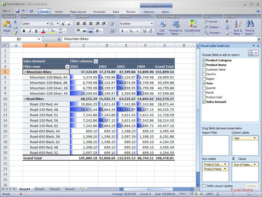
You’ll notice that there is no conditional formatting of the sales values for the “Product Category” field (“Mountain Bikes” and “Road Bikes”). It wouldn’t make much sense since those values are not at the same level as the values for the individual products.
你将注意到，在“产品品类”字段（“Mountain Bikes”和“Road Bikes”）的销售数据上没有条件格式。这没有什么意义，因为那些数据和具体产品数据不在同一个层次里。

For the sake of completeness, here is what the PivotTable would look like if I had selected All “Sum of Sales Amount” cells
为了完整起见，这里是当我选择所有“Sum of Sales Amount”单元格时的数据透视表样子。

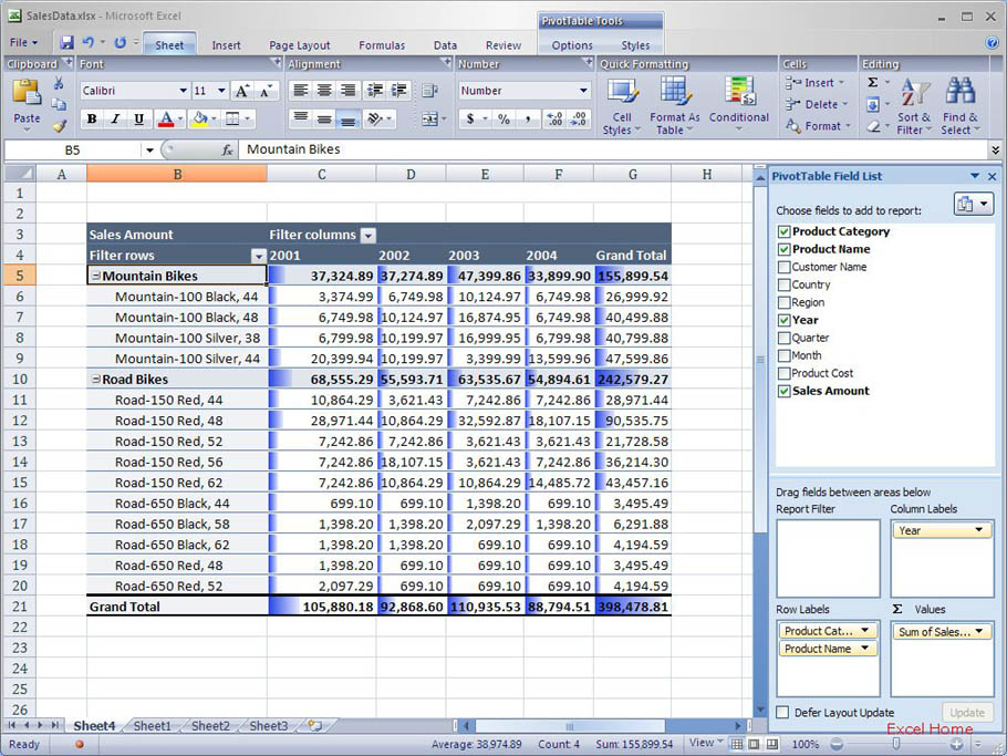
However, this doesn’t make much sense in this particular example because the grand totals skew the formatting in all the other cells so it’s hard to spot any differences. That said, this type of scoping works great for relative values, (for example % profitability) where you can directly compare values at any level of detail.
然而，在本特定示例中，这不合理，因为总计将其它所有单元格里的格式都弄乱了（译者，其它的Data bars都被迫压缩了），非常难以看出任何差别。也就是说，这种应用对于相对值很好用（例如利润百分比），你可以在任何细节层次上直接比较数值。

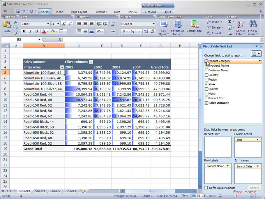
Once the conditional formatting is applied, I can interact with the PivotTable and the formatting will be reevaluated dynamically (as I mentioned above). For example, if I change my report filter to only show sales to a specific country, the sales values will be reduced to only show that information and the conditional formatting will be automatically reevaluated to reflect the new values.
一旦应用了条件格式，我可以和该数据透视表相互交流并且该格式将会动态地被重新计算（正如我在上面提到的）。例如，如果我更改报告筛选，仅显示在某个特定国家的销售，那么销售数据会减小为仅显示该信息，而条件格式会自动被重新评估来反映这些新数值。

I can also add and remove fields and have the formatting adjust to that. Here is a screenshot of the same PivotTable after having removed the “Product Category” field.
我也可以添加和删除字段，格式会随之调节。这里是一个截屏，相同的数据透视表在删除“Product Category”字段之后。

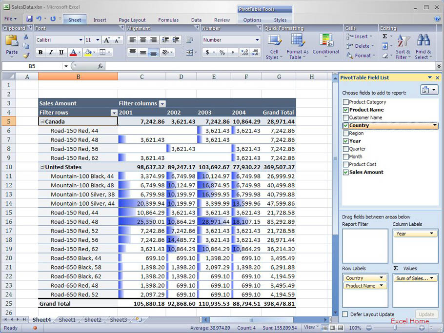
And if I add another field instead, the conditional formatting rule is automatically reevaluated again. Here is a screenshot of the PivotTable after adding the “Country” instead of the “Product Category” field I removed before.
相反，如果我添加一个字段，该条件格式规则会被重新计算。这里是个截屏，添加了“Country”字段，而不是之前删除的“Product Category”字段。

That’s the summary for conditional formatting and PivotTables. With these improvements, PivotTables can now be used as a great tool for exploring data, highlighting trends, spotting outliers, etc.
这是条件格式和数据透视表的总结。有了这些改进，数据透视表可以作为一个强大的数据研究，突出趋势，发现突出者，等等的工具来使用了。

Published Wednesday, December 21, 2005 9:57 PM by David Gainer

注：本文翻译自http://blogs.msdn.com/excel，原文作者为David Gainer(a Microsoft employee)，Excel home授权转载。严禁任何人以任何形式转载，违者必究。