技巧1_色彩缤纷的Data Bars
译者:Kevin 来源:http://blogs.msdn.com/excel
发表于:2006年7月7日
Conditional Formatting Trick 1 – Multi-Coloured Data Bars
条件格式技巧1——色彩缤纷的Data Bars
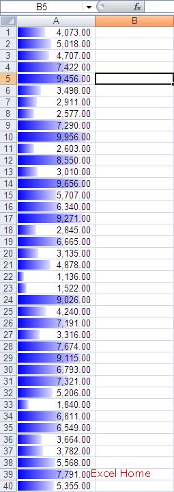
A few months ago, I described the new features we have added to Excel 2007 in the area of conditional formatting. One of the new formats we added is called a “data bar” … check out this earlier post for a refresher, but the basic idea is that Excel draws a bar in each cell representing the value of that cell relative to the other cells in the selected range. Here is a shot from that post.
几个月以前,我讲述了在Excel 2007中新增加的有关条件格式的各种特性,其中之一就是我们称之为“data bar”的……可参阅以前的文章。但是我们只讲到最基础的概念,即在一个选定的区域里面,由Excel根据不同单元格的数值对比情况,在每个单元格中绘制一个色带。下面是以前文章中的截图:
The Excel 2007 UI allows you to choose whatever colour you want for your data bars, but, by default, all the data bars you apply to a range have to be the same colour. Someone on our team recently showed me how to use a tiny bit of VBA to simulate having multiple colours of data bars on a range conditionally applied, so I thought I would pass along the trick.
Excel 2007允许你为你的data bars选择任何你想要的颜色,但是,默认情况下,同一区域中的data bars,只能有同一种颜色。最近,开发团队中的某位成员向我展示了如何在同一区域中创建多种颜色的data bars,只需要利用非常简单的VBA代码即可。所以,我想我应该好好发挥这个技巧的威力。
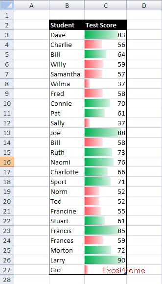
Say, for example, you are looking at student grades, and you want all the data bars for students with a passing mark (60%+ and above) to be green, and those with a failing grade (59% or less) to be red. The first thing you would do is to add some red data bars to your data, and then some green data bars. By default, Excel shows you the last set applied, so the data bars would be green. If you then launch the VB Editor (Alt + F11) and in the immediate window (Ctrl+G), type:
selection.FormatConditions(1).formula = “=if(c3>59, true, false)”
You would see that your data now looks like this, which makes it easy to spot the failing grades.
举个例子,你正在考虑为学生评分,你希望当学生成绩及格(60%或更高)时,data bars是绿色的,而不合格的成绩(59%或更低)对应的data bars是红色的。第一步,你肯定会为你的数据加上一些红色的data bars,然后是绿色的。在默认情况下,Excel只接受你最后的设置,所以所有的data bars都将是绿色的。如果你现在打开VB编辑器(Alt + F11),在立即窗口(Ctrl+G)中输入:selection.FormatConditions(1).formula = “=if(c3>59, true, false)”
你将会看到你的数据就会像下面这样,非常容易的辨识出不合格的成绩:
So how does this work? Every conditional format has a Formula property, which allows you to specify a formula which determines whether the conditional format is visible. In this case, we are simply saying that the green data bars (the most recent ones) should only be visible if a value is greater than 59.
This property is available on all conditional formats, so I expect that users will find all sorts of creative uses beyond just this case.
那么这项工作是如何完成的?原来,每一个条件格式都有一个公式的属性,此属性允许你指定一个公式来判断其本身是否可见。在这个例子中,我们简单的指定为,只有单元格数值大于59时,绿色的data bars才会被显示。
所有的条件格式都可以利用这个属性,因此,我希望用户能够发挥创造力,举一反三。
Published Friday, February 24, 2006 1:32 PM by David Gainer
注:本文翻译自http://blogs.msdn.com/excel ,原文作者为David Gainer(a Microsoft employee),Excel Home 授权转载。严禁任何人以任何形式转载,违者必究。